Joint Probability: The Basics You Need to Know
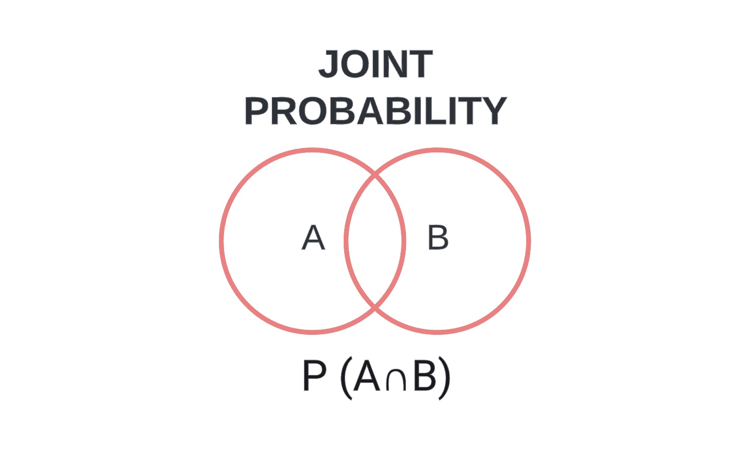
Joint probability is a fundamental concept in probability theory that describes the likelihood of two events occurring together. It is the cornerstone for understanding relationships between variables in statistics. The idea is simple: if you have two random events, what is the probability that both will happen at the same time?
This concept becomes particularly essential when dealing with multiple variables. The need to understand the joint occurrence of events underpins many practical applications such as risk assessment, data analysis, and decision-making models. Understanding joint probability can also aid in identifying correlations and dependencies among variables, which is crucial for predictive modeling.
The foundational principles of joint probability have been applied across various disciplines, ranging from finance and healthcare to machine learning and artificial intelligence. It serves as the gateway to more complex probabilistic models like conditional probability and Bayes’ Theorem.
Table Of Contents
Mathematical Representation: The Formula for Calculating Joint Probability
The joint probability measures the chance of multiple independent events happening at the same time, symbolized as P(A∩B) or P(A and B). It’s calculated by multiplying the individual probabilities: P(A) * P(B).
The mathematical formula for joint probability for two independent events A and B is P(A∩B)=P(A)×P(B). However, if the events are dependent, the formula becomes P(A∩B)=P(A∣B)×P(B), where P(A∣B) is the conditional probability of A given B.
In mathematical representation, joint probability can be shown as a table, formula, or graph. This offers flexibility for application in various types of data sets. Often, a two-dimensional matrix is used for ease of understanding when more than two events are involved.
The computation of joint probabilities serves as the basis for other vital statistical concepts like marginal probability and expected values. These elements are essential for hypothesis testing, confidence intervals, and other inferential statistics methods.
Key Concepts: Independent and Dependent Events in Joint Probability
Two events are said to be independent if the occurrence of one event does not influence the occurrence of the other. In contrast, dependent events are influenced by the occurrence of another event. Differentiating between these two is crucial for correctly applying the joint probability formula.
In cases where events are independent, each event has its own separate probability, and the joint probability is the product of these separate probabilities. For dependent events, conditional probabilities come into play, altering the formula to account for the relationship between the events.
It is often necessary to conduct a test of independence to confirm whether two events are indeed independent. This involves a variety of statistical techniques such as chi-squared tests or Fisher’s exact test. This step is critical before embarking on any advanced statistical analysis involving multiple variables.
Also Read: What is Joint Distribution in Machine Learning?
Practical Examples: Applying Joint Probability in Everyday Life
Flipping Two Coins
Scenario:
You have two coins, and you flip both of them at the same time. What is the joint probability of both coins landing heads up?
Solution:
There are 4 possible outcomes:
- Both heads (HH)
- First coin heads, second coin tails (HT)
- First coin tails, second coin heads (TH)
- Both tails (TT)
The probability of each outcome is 1/4 if we assume the coin flips are independent and fair.
The joint probability of getting both heads is 1/4.
Rolling Two Dice
Scenario:
You roll two standard six-sided dice. What is the joint probability that the first die shows a 3 and the second die shows a 4?
Solution:
There are 36 possible outcomes when you roll two dice (6 faces on the first die times 6 faces on the second die).
The event of the first die showing a 3 and the second die showing a 4 is just one event.
So, the joint probability is 1/36.
Drawing Cards from a Deck
Scenario:
You have a standard deck of 52 playing cards. You draw two cards sequentially without replacement. What is the joint probability of the first card being an Ace and the second card being a King?
Solution:
The probability of drawing the first Ace is 4/52 or 1/13.
Once an Ace is drawn, there are 51 cards left in the deck.
The probability of drawing a King next is 4/51.
The joint probability of both events happening is (1/13)×(4/51)=4/663
Health Risk Assessment
Scenario:
Based on statistical data, let’s assume that the probability of a randomly selected person being a smoker is 0.2 and the probability of a randomly selected person being obese is 0.3. Studies have shown that among the smokers, 0.1 are obese. What’s the joint probability that a randomly selected person is both a smoker and obese?
Solution:
Here, the events are dependent.
The joint probability would be P(Smoker and Obese)=P(Smoker)×P(Obese|Smoker)
=0.2×0.1=0.2×0.1
=0.02=0.02 or 2%.
These examples illustrate how joint probability can be calculated in various contexts, both with independent and dependent events.
Joint probability is often used in quality control processes in manufacturing. If there is a production line creating components, the joint probability of multiple components being defective can guide quality assurance strategies. This kind of analysis helps in deciding whether to change a manufacturing process or conduct further inspections.
Healthcare professionals use joint probability to assess the likelihood of multiple symptoms leading to a specific disease. This can be especially helpful in diagnosing complex conditions where symptoms are not exclusive to one ailment. For example, joint probabilities can be calculated to assess the risk of heart disease given factors like high cholesterol and family history.
Even in the world of finance, portfolio managers calculate the joint probabilities of different assets’ returns to optimize portfolio performance. By understanding the joint behavior of assets, they can make more informed decisions on asset allocation, thereby potentially enhancing returns while mitigating risks.
Case Studies: Joint Probability in Industry and Research
In the healthcare sector, joint probability has been utilized to create predictive models for patient outcomes. By considering multiple variables such as age, medical history, and lab results, researchers have been better able to predict the likelihood of readmission for high-risk patients. This enables more effective resource allocation within hospitals.
Joint probability plays a crucial role in cybersecurity as well. By analyzing the joint probabilities of various system vulnerabilities being exploited, security experts can prioritize which weaknesses to address first. This risk-assessment model is central to developing robust cybersecurity measures.
Machine learning algorithms often use joint probability for feature selection and data clustering. In Natural Language Processing (NLP), for example, the joint probability of certain words appearing together can significantly improve the performance of language models. This application is widely used in sentiment analysis and chatbot development.
Also Read: Introduction to Naive Bayes Classifiers
Misconceptions in Understanding Joint Probability
One of the most prevalent errors is assuming that all events are independent, thereby wrongly applying the formula for joint probability of independent events to dependent events. This can lead to inaccurate results, especially in predictive modeling where understanding the relationship between variables is crucial.
Another issue is the misuse of terminology, often confusing joint probability with other types of probabilities such as marginal or conditional probability. This confusion can affect the interpretation of data and lead to flawed conclusions.
Ignoring the possibility of mutually exclusive events is another common mistake. Events are mutually exclusive if they cannot happen at the same time. In such cases, the joint probability is zero, a fact often overlooked in various analyses which can lead to erroneous conclusions.
Joint Probability vs. Marginal and Conditional Probability
Joint probability serves as the building block for other important concepts like marginal and conditional probability. While joint probability considers the likelihood of two or more events happening together, marginal probability looks at the probability of a single event irrespective of the others.
Conditional probability, on the other hand, provides the likelihood of an event occurring given that another event has already occurred. It is a specialized form of joint probability but adjusted for the given conditions.
All three of these probabilities interrelate and complement each other. Understanding one form of probability often provides insights into the others, and they often exist side by side in complex probabilistic models.
Also Read: What is Argmax in Machine Learning?
The Role of Joint Probability in Statistics and Data Science
Joint probability is a cornerstone in the fields of statistics and data science. It forms the basis of multivariate statistical methods like multiple regression and factor analysis, often used for predictive modeling.
In data science, especially in the era of Big Data, understanding joint probability is key for machine learning algorithms and data analytics. It aids in the effective interpretation of large and complex datasets, which is crucial for decision-making in various sectors, including healthcare, finance, and technology.
The power of joint probability extends to its use in Bayesian networks, a type of probabilistic graphical model that uses Bayesian inference for probability computations. Bayesian networks are widely used in machine learning, computer vision, and robotics among other advanced technology fields.
Joint Probability Distributions and Multivariate Analysis
Beyond the basic framework, joint probability distributions provide a way to describe the likelihood of multiple events across a range of possible outcomes. For instance, the joint normal distribution extends the idea of a normal distribution to multiple variables.
Multivariate analysis uses joint probability as a fundamental concept to analyze more than two variables simultaneously. This is crucial in complex systems where multiple factors interact with each other, such as in econometrics, multivariate testing in marketing, or genomic analysis in bioinformatics.
Markov Chains and Hidden Markov Models are advanced models that use joint probabilities to predict future states based on current and past states. They have applications ranging from stock market prediction to natural language processing and are an extension of joint probability theory.
Key Takeaways and Best Practices in Using Joint Probability
Understanding the fundamentals of joint probability is crucial for anyone involved in statistical analysis or data science. It not only aids in understanding relationships between variables but also serves as a gateway to more complex statistical methods.
Best practices in using joint probability involve careful identification of dependent and independent events, proper use of formulas, and judicious application in practical problems. A sound understanding of joint probability is often the first step in creating accurate and reliable predictive models.
Being aware of common mistakes can also be beneficial. Always test for independence before proceeding with calculations and be clear on the distinctions between joint, marginal, and conditional probabilities to ensure that you are applying the correct formula and interpretation.


