

Introduction
Radial Basis Function Networks (RBFNs) offer a unique approach to neural networks that has piqued the interest of researchers and practitioners alike.
Known for their unique properties and advantages, Radial bias function networks have become increasingly popular in applications such as pattern recognition, function approximation, and time series prediction. We will take you through an in-depth exploration of the RBFN architecture, its underlying concepts, and the training process. To further enhance your understanding, we will discuss practical examples, address frequently asked questions, and examine the benefits of employing RBFNs in various scenarios.
What Are Radial Basis Functions?
Radial Basis Functions (RBFs) are mathematical functions used to approximate complex, continuous functions. They are characterized by their radial symmetry, meaning that their value depends only on the Euclidean distance between input points and a center point.
In simpler terms, Radial Basis Function (RBF) is a function whose output changes based on how far the input is from the center point. RBFs are symmetric around their center, meaning the output remains the same if the distance from the center is the same, regardless of the direction.

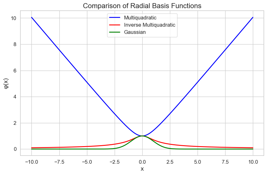
Multiquadratic, inverse multiquadratic, and Gaussian functions are different types of radial basis functions used in various applications. Let’s briefly describe each of them:
Multiquadratic Function
The multiquadratic function is given by:
φ(x) = √(‖x – c‖^2 + R^2)
where x is the input vector, c is the center of the function, and R is a constant parameter.
Inverse Multiquadratic Function
The inverse multiquadratic function is given by:
φ(x) = 1 / √(‖x – c‖^2 + R^2)
Gaussian Function
An example of an RBF is the Gaussian function, which is characterized by a width or scale parameter (a). This parameter determines how “wide” the function is, affecting how quickly the output changes as the distance from the center increases.
An RBF can be written as:
Φc(x) = Φ(||x – μc||; a) (1)
Here, Φc(x) is the RBF, x is the input, μc is the center, || · || is a vector norm (e.g., Euclidean norm), and a is the width parameter.

Radial Basis Function Networks (RBFNs) involve several key equations in their formulation, training, and operation. Here, we will outline the main equations step by step:
RBFs can be combined to represent more complex functions by using them as a basis for linear combinations:
y(x) = Σ(wjΦ(||x – μj||)) (2)
In this equation, y(x) is the output function, wj are the weights for each RBF, and the summation goes from 1 to M, where M is the total number of RBFs used.
Also Read: What is Transfer Learning And How Is It Used In Machine Learning?
What Are Radial Basis Function Networks and how do they work?
A Radial Basis Function Network (RBFN) is a type of feedforward neural network that uses RBFs in its hidden layer. The network consists of three layers: the input layer, the hidden/kernel layer, and the output layer.
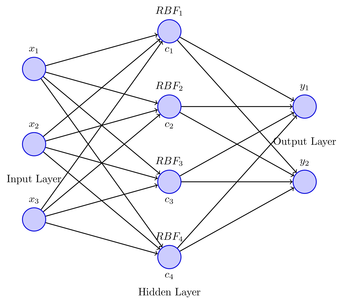
The input layer receives an n-dimensional input vector, and each node in the hidden layer represents RBF neurons that are centered at a specific point in the input space. The output layer combines the outputs of the hidden layer nodes through a linear combination of weights to generate the final output values.
RBF Network Architecture
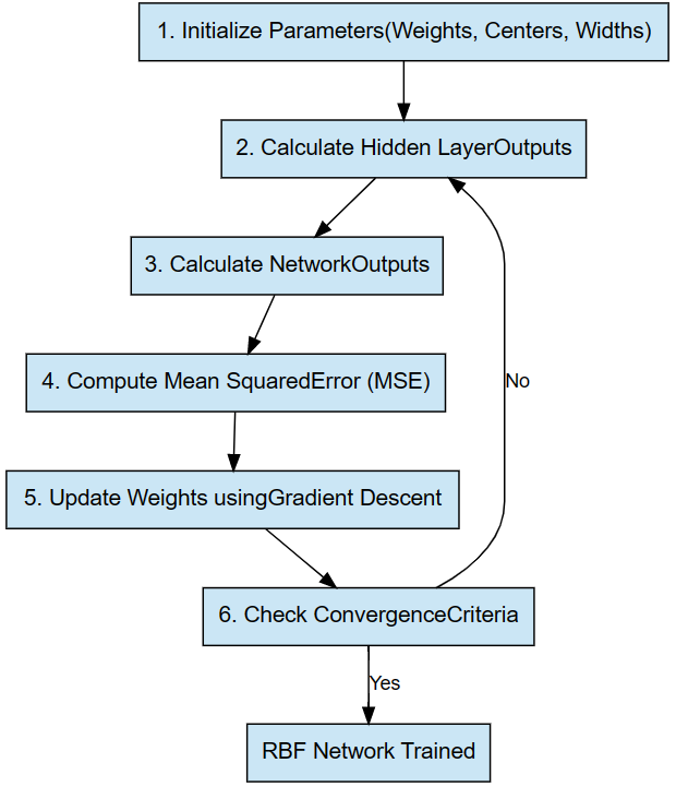
Flowchart illustrating the RBF Network Training Process, including initialization of parameters, computation of hidden layer outputs and network outputs, evaluation of Mean Squared Error (MSE), weight updates using gradient descent, and convergence checks.
Input Layer
The input layer consists of input neurons that receive input values and pass them to the hidden layer. The number of input neurons corresponds to the dimensionality of the input vector.
Hidden Layer
The hidden layer is composed of hidden units or computational units that apply the Radial Basis Function (RBF), such as the Gaussian function, to the input values. Each hidden unit calculates the Euclidean distance between the input vector and its center and applies the RBF to this distance. The number of hidden units determines the network’s capacity for function approximation:
h_j(x) = φ(‖x – c_j‖)
where h_j(x) is the output of the j-th hidden unit, c_j is the center vector associated with the j-th hidden unit, and φ(‖x – c_j‖) is the RBF.
Output Layer
The output layer contains output neurons that generate output values through a linear combination of the hidden layer outputs and the matrix of output weights. The number of output neurons depends on the desired dimensionality of the output vector.
y_k(x) = Σ_j w_jk * h_j(x)
where y_k(x) is the k-th output of the network, w_jk is the weight connecting the j-th hidden unit to the k-th output neuron, and h_j(x) is the output of the j-th hidden unit.
Now let’s discuss the Radial Basis Function (RBF) network mapping equation, which can be represented as:
y(x) = Σ_j w_j * φ(||x – μ_j||)
To simplify the equation, we can introduce an extra basis function φ0(x) = 1:
y(x) = w_0 + Σ_j w_j * φ(||x – μ_j||)
Here, we have M basis centers (μj) and M widths (σj). In the next section, we will discuss how to determine all the network parameters (wkj, μj, and σj).
Training the Radial Bias Function Networks
Mean Squared Error (MSE)
During training, the objective is to minimize the mean squared error between the network’s output and the target output for a given set of training examples:
MSE = (1/N) Σ_n (t_kn – y_k(x_n))^2
where N is the number of training examples, t_kn is the target output for the k-th output neuron and the n-th example, and y_k(x_n) is the network’s output for the k-th output neuron and the n-th example.
Weight Update Rule (Gradient Descent)
When using gradient descent to learn the output weights, the weight update rule is as follows:
w_jk(t+1) = w_jk(t) – η * ∂MSE/∂w_jk
where w_jk(t) is the weight connecting the j-th hidden unit to the k-th output neuron at iteration t, η is the learning rate, and ∂MSE/∂w_jk is the partial derivative of the mean squared error with respect to the weight w_jk.
Radial Basis Function Neural Network Example
import numpy as np
import matplotlib.pyplot as plt
from sklearn.datasets import make_moons
from sklearn.neural_network import MLPClassifier
from sklearn.pipeline import make_pipeline
from sklearn.preprocessing import StandardScaler
from sklearn.svm import SVC
from matplotlib.colors import ListedColormap # Generate toy dataset
X, y = make_moons(n_samples=300, noise=0.05, random_state=42) # Create ANN and RBFN models
ann = make_pipeline(StandardScaler(), MLPClassifier(hidden_layer_sizes=(100,), max_iter=500, random_state=42))
rbfn = make_pipeline(StandardScaler(), SVC(kernel='rbf', C=1, gamma=1)) models = [('ANN', ann), ('RBFN', rbfn)] # Plot the dataset and decision boundaries
fig, axes = plt.subplots(1, 3, figsize=(15, 5))
cm = plt.cm.RdBu
cm_bright = ListedColormap(['#FF0000', '#0000FF'])
titles = ['Moon Dataset', 'ANN Decision Boundary', 'RBFN Decision Boundary'] # Plot the dataset
axes[0].scatter(X[:, 0], X[:, 1], c=y, cmap=cm_bright, edgecolors='k', s=50)
axes[0].set_xlim(X[:, 0].min() - .5, X[:, 0].max() + .5)
axes[0].set_ylim(X[:, 1].min() - .5, X[:, 1].max() + .5)
axes[0].set_xticks(())
axes[0].set_yticks(())
axes[0].set_title(titles[0]) # Train and plot decision boundaries for ANN and RBFN
for (name, model), ax, title in zip(models, axes[1:], titles[1:]):
model.fit(X, y)
x_min, x_max = X[:, 0].min() - .5, X[:, 0].max() + .5
y_min, y_max = X[:, 1].min() - .5, X[:, 1].max() + .5
xx, yy = np.meshgrid(np.arange(x_min, x_max, 0.02), np.arange(y_min, y_max, 0.02))
Z = model.predict(np.c_[xx.ravel(), yy.ravel()])
Z = Z.reshape(xx.shape)
ax.contourf(xx, yy, Z, cmap=cm, alpha=.8)
ax.scatter(X[:, 0], X[:, 1], c=y, cmap=cm_bright, edgecolors='k', s=50)
ax.set_xlim(x_min, x_max)
ax.set_ylim(y_min, y_max)
ax.set_xticks(())
ax.set_yticks(())
ax.set_title(title) plt.tight_layout()
plt.savefig('ANN_RBFN_comparison.png', dpi=300)
plt.show()

Comparing Artificial Neural Networks (ANN) and Radial Basis Function Networks (RBFN) for Nonlinear Classification: A Visual Demonstration on the Moon Dataset”
Advantages of RBFN
Faster learning speed: RBFNs generally require fewer iterations during training, as the training process is divided into separate stages for learning the RBF centers and output weights. It also requires less extensive hyperparameter tuning than other MLP networks.
Universal approximation capability: Radial bias function networks are known as universal approximators, meaning they can approximate any continuous function with arbitrary accuracy, given a sufficient number of hidden units.
Localized processing: Radial bias function networks employ locally-tuned processing units, which can lead to improved generalization performance, especially in tasks where the input data exhibits local structure or patterns.
Also Read: Introduction to PyTorch Loss Functions and Machine Learning
FAQ’s
What is the role of the radial basis?
The radial basis function serves as the activation function for the hidden layer units in an RBFN, determining the output of each hidden unit based on the input vector’s Euclidean distance from the RBF center.
What is the radial basis function in ML?
In ML, radial basis functions are used as basis functions for function approximation, kernel methods, and as activation functions in RBFNs, enabling the network to learn complex, non-linear relationships between input and output data.
What is the difference between RBF and MLP?
RBFNs offer several advantages, including faster learning speed, universal approximation capability, and localized processing, which can lead to improved generalization performance in tasks involving local patterns or structures in the input data.
What is the difference between RBF and MLP?
A: RBFNs and MLPs are both feed-forward neural networks, but they differ in their activation functions and training processes. RBFNs use radial basis functions as activation functions in the hidden layer and typically have a two-stage training process, while MLPs use other types of activation functions (e.g., sigmoid or ReLU) and employ backpropagation for training.
Also Read: Rectified Linear Unit (ReLU): Introduction and Uses in Machine Learning
Conclusion
In conclusion, Radial Basis Function Networks (RBFNs) carve a distinctive niche within the realm of neural networks by utilizing radial basis functions as activation functions in their hidden layers. Their architecture, with an emphasis on local structure and patterns, grants RBFNs a competitive edge in domains such as function approximation, pattern recognition, and time series prediction. This article has provided a comprehensive overview of RBFNs, their underlying concepts, and the training process, along with practical examples to further enhance the understanding of these networks.
References
Ghosh, and Nag. “An Overview of Radial Basis Function Networks.” Physica-Verlag HD, 1 Jan. 2001, https://link.springer.com/chapter/10.1007/978-3-7908-1826-0_1. Accessed 20 Apr. 2023.
Ramadhan, Luthfi. “Radial Basis Function Neural Network Simplified.” Towards Data Science, 10 Nov. 2021, https://towardsdatascience.com/radial-basis-function-neural-network-simplified-6f26e3d5e04d. Accessed 20 Apr. 2023.
Simplilearn. “What Are Radial Basis Functions Neural Networks? Everything You Need to Know.” Simplilearn, 5 Sept. 2022, https://www.simplilearn.com/tutorials/machine-learning-tutorial/what-are-radial-basis-functions-neural-networks. Accessed 20 Apr. 2023.