Introduction
Support Vector Machines (SVMs) are a class of supervised learning models and associated training algorithms that were founded on statistical learning theory. They were discovered in the 90s at the AT&T Bell Laboratories by Vladmir Vapnik and his colleagues and are considered one of the most robust and popular classification algorithms in machine learning.
In this article, we will learn about the concepts, the math and the implementation of support vector machines. The outline is as follows. We will review the background on linear classifier and maximal margin and soft margin classification. We will then outline the concept of support vector machines and kernel functions. The math behind SVMs will be reviewed, followed by implementation aspects in the Python Scikit-Learn library. We will conclude by summarizing the article and comparing it to other supervised machine learning algorithms.
Table of contents
Background
Let’s consider a simple 1-dimensional 2-class classification problem: assigning a risk category, high-risk or low-risk, to loan applicants based on just their credit scores. The credit scores in the US typically range from 300 – 850 and the goal is to assign a binary label based on a threshold value. The training examples, which are shown in the figure below consist of few examples of each category. Three possibilities for the decision threshold are also illustrated.

The first case on the left draws the decision boundary dangerously close to the high-risk training data. The chance of classifying a test data point that is statistically closer to the high-risk subset of training points, as low-risk is significant. Most likely, this will be a misclassification. Similarly, the decision boundary on the right runs the risk of misclassifying test data in the other direction: data points that are statistically closer to low-risk class will be classified as high-risk. The decision boundary shown in the middle is drawn at the mid-point between the positive and negative training data, thereby maximizing the margins in both directions. Any test data point will be classified purely on the basis of its statistical closeness to the training data from the respective class. In other words, this is the most reasonable decision function that will maximize the model performance. Such a classification rule is called a maximum margin classifier and it provides the most optimal class prediction.
Unfortunately, the maximal margin approach has a major disadvantage: it is sensitive to outliers. Consider the situation shown below, where we have an outlier high risk data point in the training samples.
The outlier data point will significantly reduce the margin and result in a classifier that fails to mitigate the bias-variance tradeoff. It will work very well on training data, thereby having high variance, but will fail on unseen test data, resulting in low bias. We need to maximize the margins, but also generalize well to unseen test data. Moreover, the blue high-risk data point may not even be an outlier. The data may generally have some overlap and may not be cleanly separated as shown in the above figures. In such cases, soft margin classifiers are the solution to maximizing the real-world model performance!
Soft margin classifiers, also known as support vector classifiers, allow training data to be misclassified, thereby improving the ability of the model to handle outliers and generalize to unseen data. As shown below, the soft margin classifier will allow the outlier training sample to mis-classifed and choose the decision boundary somewhere in the middle. The exact location of the decision boundary is optimized using cross – validation. Multiple folds of data will be used to tune the decision boundary in such a way that optimizes the bias-variance tradeoff.
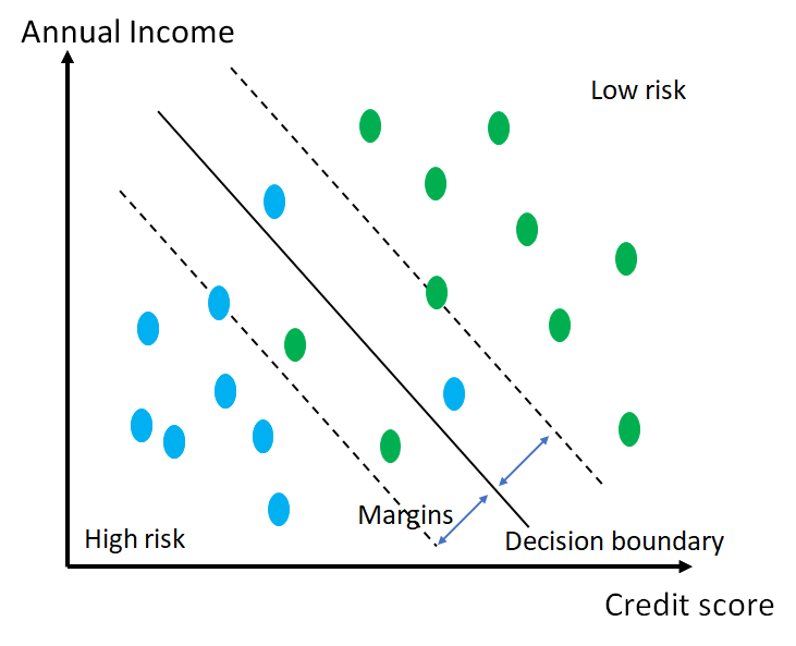
The above example was in a single dimensional space. We visualize support vector classifier in 2 and 3 dimensional spaces below. In the 2-dimensional example, we the annual income of the applicant is added ad an additional feature to the problem of estimating loan risk class. In the 3-dimensional case,, the applicant’s age is the additional feature. In the 3-dimensional version, the smaller data points are further along the age-axis and denote older applicants. The decision function increases in dimensionality as we increase the additional features. In the 1-dimensional case, it was a point, in the 2-dimensional case, we have a line and in the 3-dimensional case, a plane is used to separate the two classes. In the (N+1)-dimensional space, the decision function will be an N dimensional hyperplane.
 |
|
| Support vector classifiers in multidimensional spaces: in the 3D case, the smaller points are further into the third axis (Age) and therefore represent older applicants in the training set. | |
Soft margin classifiers increase the classification performance on unseen data, thereby improving the bias-variance tradeoff in the real-world. Support vector machines are further generalizations of support vector classifiers in that they i) allow soft margin classification and ii) can handle much higher overlap between the classes using nonlinear kernel functions. We begin by understanding the math behind support vector classification.
Also Read: Top 20 Machine Learning Algorithms Explained
Hyperplanes and Support Vectors
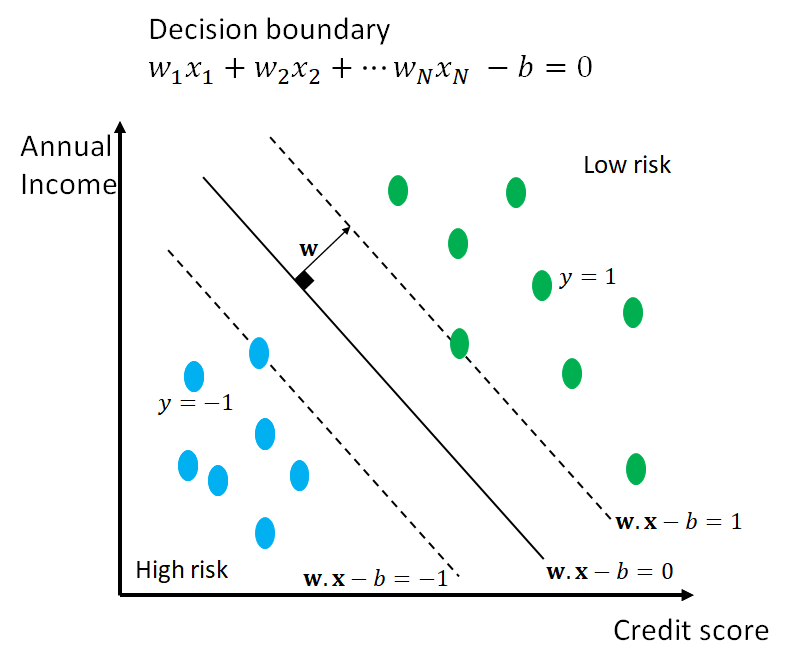
In this section, we will formulate the hard-margin version of the support vector classification. It will be generalized to the soft-margin case in the subsequent section. The figure below shows a 2-dimensional version of our binary classification problem. The training set is given by the points shown in the figure and each have a corresponding labels +1 (low risk) or -1 (high risk). The goal is the decide the decision boundary that separates data into the two target classes.

The decision boundary is shown in the black solid line. The dashed lines pass through the support vectors and define the margin boundaries for classification. The goal of fitting a support vector machine classifier is to find a “good” decision boundary, which is defined generally as a hyperplane in an N-dimensional space. As shown in the figure, the hyper – plane is defined by 1) the vector of coefficients w and 2) the intercept b. In our 2D case, w has just 2 coefficients. Thus, the problem of finding a good decision boundary boils down to finding good values for w and b of the hyperplane.
To quantify the goodness of the decision boundary, we impose the following conditions on the support vectors and the margins. The decision plane, when moved to the support vector on the +1 side takes the value 1. Conversely, when the plane is moved to the support vector on the -1 side, it takes the value -1. By definition, any point on the decision boundary evaluates to 0. We have now transformed the problem of finding a good decision boundary to estimating the values of w, the vector of coefficients and b, such that the aforementioned conditions are met, and the gap between the two classes is maximized. Next, we will formulate the optimization problem that encodes these conditions.
The normal vector to the hyperplane decision boundary is defined by the vector of coefficients w of the hyperplane itself! So the first thing to do is to consider a unit vector in the direction w. Then, we can ask: starting at the decision boundary, how much do I have to walk in the direction of this unit vector to reach the support vectors in either direction. This quantifies the margin for the binary classifier. We know that a point x on the decision boundary must satisfy w.x – b = 0 and when it reaches the corresponding points on the support vectors (dashed lines) it must satisfy w.x – b = 1 and w.x – b = -1 respectively. The amount of translation needed to reach the two dashed lines can be expressed a scalar multiple k of the unit vector as follows.
Thus, the margin is given by 2(1/||w||) as it symmetric in both directions. As we mentioned earlier, the goal is to maximize the margin in both directions. Thus minimizing ||w|| will be the objective our our optimization problem.
The constraints are based on further moving the hyperplane in both the directions. As we move the hyperplane further into the +1 space (green points), we constrain the points to evaluate to >=1. Similarly, when the hyperplane is moved further into the -1 space (blue points), we constrain the points to evaluate to <= -1. These can be formalized as below.
We are now ready to express our optimization problem in terms of the training data. Consider that we have N training vectors x_i, along with their class labels y_i. Then, the goal is to find the vector of coefficients w and b, such that the following problem is optimized.
Soft and Large Margin Intuition
Next, we generalize the problem formulation to the case of soft margins, which allows for misclassifications, thereby achieving a better generalization in the real world, where the data is not cleanly separated. We show such a scenario in the figure below, with some data points in the training set within the decision boundary and one outlier that has been misclassified.
The hinge loss function, which is depicted below, is crucial to the soft margin formulation. Let’s imagine the hinge loss function for the four training examples marked A, B, C and D in the figure above.
The data point A has the true label of +1 and the class prediction based on the decision boundary is correct. The hinge loss evaluates to max[0, 1 – 1(w.x – b)], where w.x – b will be more than 1. Remember that the hyperplane takes the value 1 at the support vector and then increases as we move further into the space of low-risk data points. Therefore, the second term will be negative, causing the hinge loss to be 0. This is reasonable as we do not want the correctly classified data points to add to the overall loss.
Next, let’s consider the data point B. It is similar to the case above as the decision boundary correctly classifies it as -1. In this case, the hinge loss evaluates to max[0, 1 – (-1)(w.x – b)], where w.x – b will be less than 1, again making the second term negative.
Now, let’s consider the point C. It is of high-risk (-1) category, but is mis-classified by the decision boundary as +1. The hinge loss in this case will be max[0, 1 – (-1)(w.x – b)], where w.x – b will be more than 1. Therefore the second term will be positive, resulting in a non-0 loss more than 1. This is a data point that is on the left of the y-axis in the hinge loss plot above.
Finally, let’s consider the data point D. It is correctly classified by the decision boundary, but it lies within the margin and therefore is too close for comfort. The hinge loss will be max[0, 1 – 1(w.x – b)], where w.x – b will be positive, but less than 1. This will result in a loss that is less than 1, but still non-0. This is a data point on the right of the y-axis on the inclined line, in the hinge loss plot above.
Based on the above examples, we see that the hinge loss is perfectly suited for the soft-margin version of the linear classifier.
Cost Function and Gradient Updates
We are now ready to formulate the soft-margin version for support vector machines.

Next, we will unpack the two terms of the cost function. The first term is just the average hinge loss across the training set. The vector of coefficients w and the scalar value b must be chosen such that the average hinge loss across the training set is minimized. This not only ensures that any data point that is misclassified is contributing significantly to the cost function, but also ensures that the number of points lying within the margin are minimized. The second term is similar to the hard margin version and is intended to maximize the separability between the two classes.
The term lambda is a regularization parameter and it allows us to tune the importance given to the two terms. Such regularization parameters are used to tradeoff between two potentially conflicting objectives, or to choose the simplest possible solution.
Typically, numerical techniques, like gradient descent, are used to to solving this optimization problem within a training algorithm. We can analyze the partial derivatives of the cost function with respect to the coefficients to understand how gradient descent would work on the training set.

In the above equations, w_k and x_ik are the kth components of the corresponding vectors. As we can see, if a data point is correctly classified, the partial derivative only involves the regularization parameter and the kth entry from the vector of coefficients. In this case, the gradient decent update would simply be as follows.
When the data point is incorrectly classified, we also need to account for the contribution from the hinge loss term.
In these update equations, alpha represents the learning rate.
Now, we are ready to take the next step in the SVM story. Note that we have been talking of linear separation between the data points, which results in hyperplane decision boundaries. This is a strong assumption and often in the real world, data is not cleanly separable, even with soft-margin linear classification. The notion of a kernel becomes important here. Kernel functions transform the data into higher dimensional spaces, where a linear hyperplane can separate the classes effectively. Kernel functions are often nonlinear in nature, resulting in the final SVM becoming a nonlinear classifier. Our discussion thus far has been a special case and used the linear kernel. A linear kernel does not transform the data to a higher-dimensional basis. In the nonlinear case, the kernel parameters get added to the problem of fitting an SVM classifier. A full discussion is out of scope of this article.
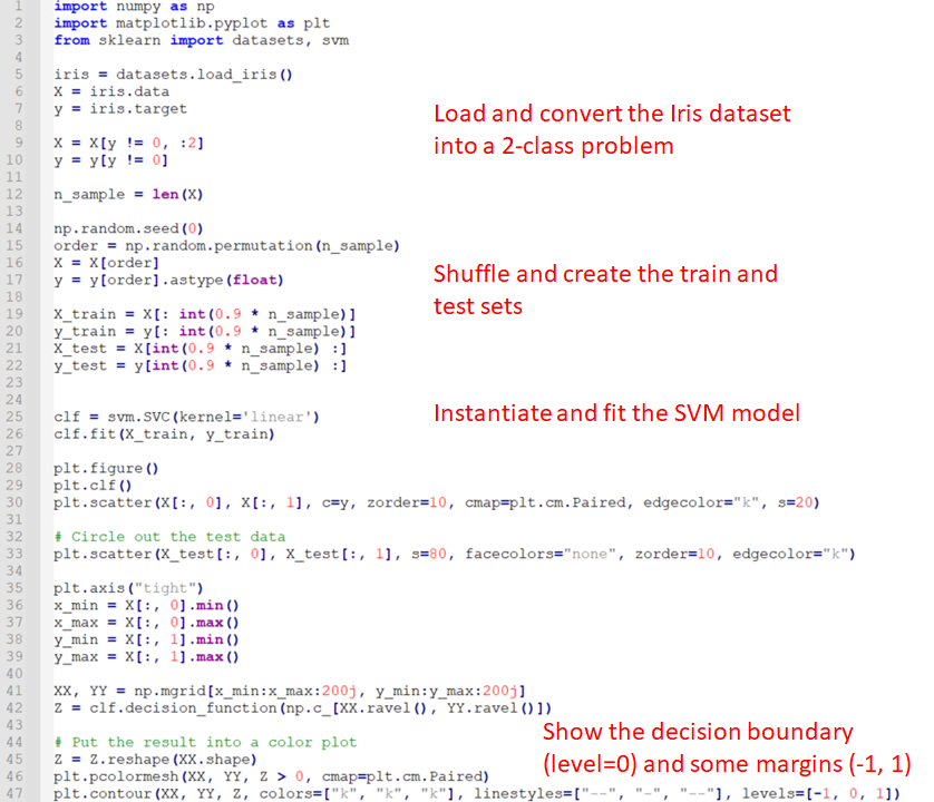
We provide some starter code based on this exercise to understand the implementation of SVMs in Python. The example creates a binary classification problem from the Iris dataset. A linear SVM classifier is then fit on the training portion of the data. Note that the only hyper – parameter is the type of the kernel.

The data and the resulting SVM classifier is visualized in the later lines. The resulting figure is shown below.
The training data is shown as circular points, whereas the test data appear as rings. The decision boundary and the margins are plotted in solid black and dashed lines respectively by line 47 in the code above. We can see the soft-margin nature of the classifier, in that it allows for misclassifications on either side of the decision boundary.
Applications of SVM
Support vector machines have found several successful applications from gene expression data analysis to breast cancer diagnosis.
1. Gene expression monitoring and analysis has been successfully carried out using SVMs to find new genes, which can then form the basis of diagnosing and treating genetic diseases.
2. Classification of cancer vs non-cancer images enables the early diagnosis of breast cancer. Google AI proved the feasibility of accurate classification of cancer images in 2020.
3. SVMs are also very good at spam mail detection and online learning methods have been created in the literature.
Advantages of using SVM
1. Support vector machines can handle high-dimensional datasets, on which it may be difficult to perform feature selection for dimensionality reduction.
2. SVMs are memory efficient: only the vector of coefficients need to be stored in memory.
3. The soft-margin approach of SVMs makes then robust to outliers.
Challenges of using SVM
1. The training time of the SVM algorithm is high, and therefore the algorithm doesn’t scale to very large datasets. Reduction of the SVM training time is an active area of research.
2. Despite the low generalization error of the soft-margin classifier, the overall interpretability of the results may be low due to the transformations induced by the nonlinear classifier components like the kernel function.
2. The choice of the kernel and regularization hyper – parameters makes the training process complex. Cross – validation is the typical solution.
Also Read: Introduction to PyTorch Loss Functions and Machine Learning
Conclusion
In this article, we reviewed the famous SVM classifiers. Based in statistical learning theory, they are one of the most popular machine learning algorithms. The concepts of hard and soft margin classifiers were detailed, building up to the formulation of the soft margin optimization problem for fitting an SVM. A small example of a linear SVM implementation in Python was also provided. Despite the reduced interpretability, which is a strong point in decision trees, they scale well to higher dimensions without easily getting overfit. SVMs share the aspect of approximating the decision boundary with nonlinear functions with neural networks, but need significantly lesser data to train. Neural networks on the other hand have more complex nonlinear interactions and therefore approximate much more complex decision boundaries.
References
Murty, M. N., and Rashmi Raghava. Support Vector Machines and Perceptrons: Learning, Optimization, Classification, and Application to Social Networks. Springer, 2016.
Soman, K. P., et al. Machine Learning with SVM and Other Kernel Methods. PHI Learning Pvt. Ltd., 2009.
Wang, Lipo. Support Vector Machines: Theory and Applications. Springer Science & Business Media, 2005.


